
In a prevous part of the course, we saw that binomial probabilites could be used to solve problems such as "If a fair coin is flipped 2 times, what is the probability of getting 2 heads?" The probability of exactly k heads out of N flips can be computed using a formula OR using an online calculator here:
If we want to know the probability of a certain number of heads or more, the problem is a bit more difficult to solve. To solve this kind of problem for a large N (say 100) and a large number of heads (say 60), you compute the probability of 60 heads, then the probability of 61 heads, 62 heads, etc., and add up all these probabilities. Imagine how long it must have taken to compute binomial probabilities before the advent of calculators and computers!
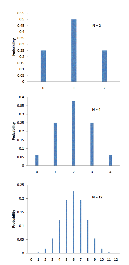
Abraham de Moivre, an 18th century statistician and consultant to gamblers, was often called upon to make these lengthy computations. de Moivre noted that when the number of events (coin flips) increased, the shape of the binomial distribution approached a very smooth curve. Binomial distributions for 2, 4, and 12 flips are shown in Figure 1.

Figure 1. Examples of binomial distributions. The heights of the blue bars represent the probabilities.
de Moivre reasoned that if he could find a mathematical expression for this curve, he would be able to solve problems such as finding the probability of 60 or more heads out of 100 coin flips much more easily. This is exactly what he did, and the curve he discovered is now called the "normal curve."

Figure 2. The normal approximation to the binomial distribution for 12 coin flips. The smooth curve is the normal distribution. Note how well it approximates the binomial probabilities represented by the heights of the blue lines.
The importance of the normal curve stems primarily from the fact that the distributions of many natural phenomena are at least APPROXIMATELY normally distributed. One of the first applications of the normal distribution was to the analysis of errors of measurement made in astronomical observations, errors that occurred because of imperfect instruments and imperfect observers. Galileo in the 17th century noted that these errors were symmetric and that small errors occurred more frequently than large errors. This led to several hypothesized distributions of errors, but it was not until the early 19th century that it was discovered that these errors followed a normal distribution. Independently, the mathematicians Adrain in 1808 and Gauss in 1809 developed the formula for the normal distribution and showed that errors were fit well by this distribution.
This same distribution had been discovered by Laplace in 1778 when he derived the extremely important central limit theorem, the topic of a later section of this reading. Laplace showed that even if a distribution is not normally distributed, the means of repeated samples from the distribution would be very nearly normally distributed, and that the larger the sample size, the closer the distribution of means would be to a normal distribution.
Most statistical procedures for testing differences between means assume normal distributions. Because the distribution of means is very close to normal, these tests work well even if the original distribution is only roughly normal.
Quételet was the first to apply the normal distribution to human characteristics. He noted that characteristics such as height, weight, and strength were normally distributed.
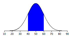
Areas under portions of a normal distribution can be computed by using calculus. Since this is a non-mathematical treatment of statistics, we will rely on computer programs and tables to determine these areas. Figure 3 shows a normal distribution with a mean of 50 and a standard deviation of 10. The shaded area between 40 and 60 contains 68% of the distribution.

Figure 3. Normal distribution with a mean of 50 and standard deviation of 10. 68% of the area is within one standard deviation (10) of the mean (50).
Figure 4 shows a normal distribution with a mean of 100 and a standard deviation of 20. As in Figure 3, 68% of the distribution is within one standard deviation of the mean.

Figure 4. Normal distribution with a mean of 100 and standard deviation of 20. 68% of the area is within one standard deviation (20) of the mean (100).
The normal distributions shown in Figures 3 and 4 are specific examples of the general rule that 68% of the area of any normal distribution is within one standard deviation of the mean. Rules you should know are:
1) 34% of the area under a normal distribution is between the mean and 1 standard deviation above the mean
2) 14% of the area under a normal distribution is between the 1 and 2 standard deviations above the mean
3) 2% of the area under a normal distribution is more than 2 standard deviations above the mean
A normal calculator can be used to calculate areas under the normal distribution. For example, you can use it to find the proportion of a normal distribution with a mean of 90 and a standard deviation of 12 that is above 110. Set the mean to 90 and the standard deviation to 12. Then enter "110" in the box to the right of the radio button "Above." At the bottom of the display you will see that the shaded area is 0.0478. See if you can use the calculator to find that the area between 115 and 120 is 0.0124.

Figure 5. Display from calculator showing the area above 110.
Below is a link to the normal calculator. Use it to verify the three rules above. Try it out!
Below is a video of the information covered in this reading. Go ahead and check it out.